using the Poisson distribution to guess how many streak-freezes I'll use over the next 4 months

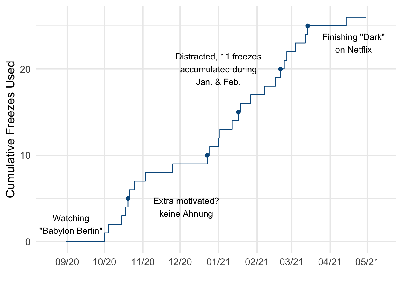
So, this is a small thing, but something I’m proud of. Over the past year, I’ve been practicing German (🇩🇪 Ich habe Deutsch gelernt!) using Duolingo’s mobile app. I don’t have an especially romantic reason for why I settled on the language, but I had watched the first season of Dark on Netflix in 2018, and don’t really enjoy dubbed foreign film/tv. Listening to the language prompted me to try a few lessons initially, but I settled into routine practice while finishing Babylon Berlin¹ last fall. I don’t remember setting an explicit goal to reach a year of daily practice, but we’re coming up on that point. According to the app, I’ve been on a streak of 217 days! Leider habe ich nicht jeden Tag geübt. There were several days where I missed my usual 20-25 minutes of practice, but Duolingo lets you purchase “streak freezes” with in-app currency to preserve your progress. Here’s a snapshot of my streak(s) over the past 8 months.

So, each freeze is a day that I’m “behind” on my goal. If I’ve used 26 freezes now, how many more should I expect over the next 4-ish months? I started right around the end of August, so 17 weeks from now would be close to my 1-year mark of daily practice. When counting the number of freezes on a weekly basis, the distribution looks fairly close to a Poisson distribution.

# I've omitted my prep code-- 'dates' is a dataset with 1 row/day,
# and an indicator 0/1 for whether a streak-freeze was used on a given day.
data.frame(dates)[1:3, ]

##         date freeze     mon wk
## 1 2020-08-31      0 Aug '20  1
## 2 2020-09-01      0 Sep '20  1
## 3 2020-09-02      0 Sep '20  1

weekly <- dates %>%
  group_by(wk) %>%
  tally(freeze)

weekly %>%
  summarise(wk = max(wk), m = mean(n), v = var(n), min = min(n), max = max(n)) %>%
  kable(col.names = c("# Weeks", "Mean", "Variance", "Min.", "Max."), digits = 3)

# Weeks	Mean	Variance	Min.	Max.
36	0.722	0.778	0	3

library(distributions3)

compare_w_poisson <- weekly %>%
  count(n) %>%
  mutate(p = nn / sum(nn), poi = pmf(Poisson(0.722), n)) %>%
  pivot_longer(p:poi)

ggplot(compare_w_poisson, aes(x = n, y = value, fill = name)) +
  geom_col(position = "dodge") +
  geom_text(aes(label = round(value, 2)), position = position_dodge(1), vjust = -0.25) +
  scico::scale_fill_scico_d(name = "", palette = "nuuk", labels = c("p" = "Observed Proportion", "poi" = "Poisson Probability (&lambda; = 0.722)")) +
  labs(x = "# freezes used during a given week", y = "") +
  theme(legend.position = "top", legend.text = ggtext::element_markdown())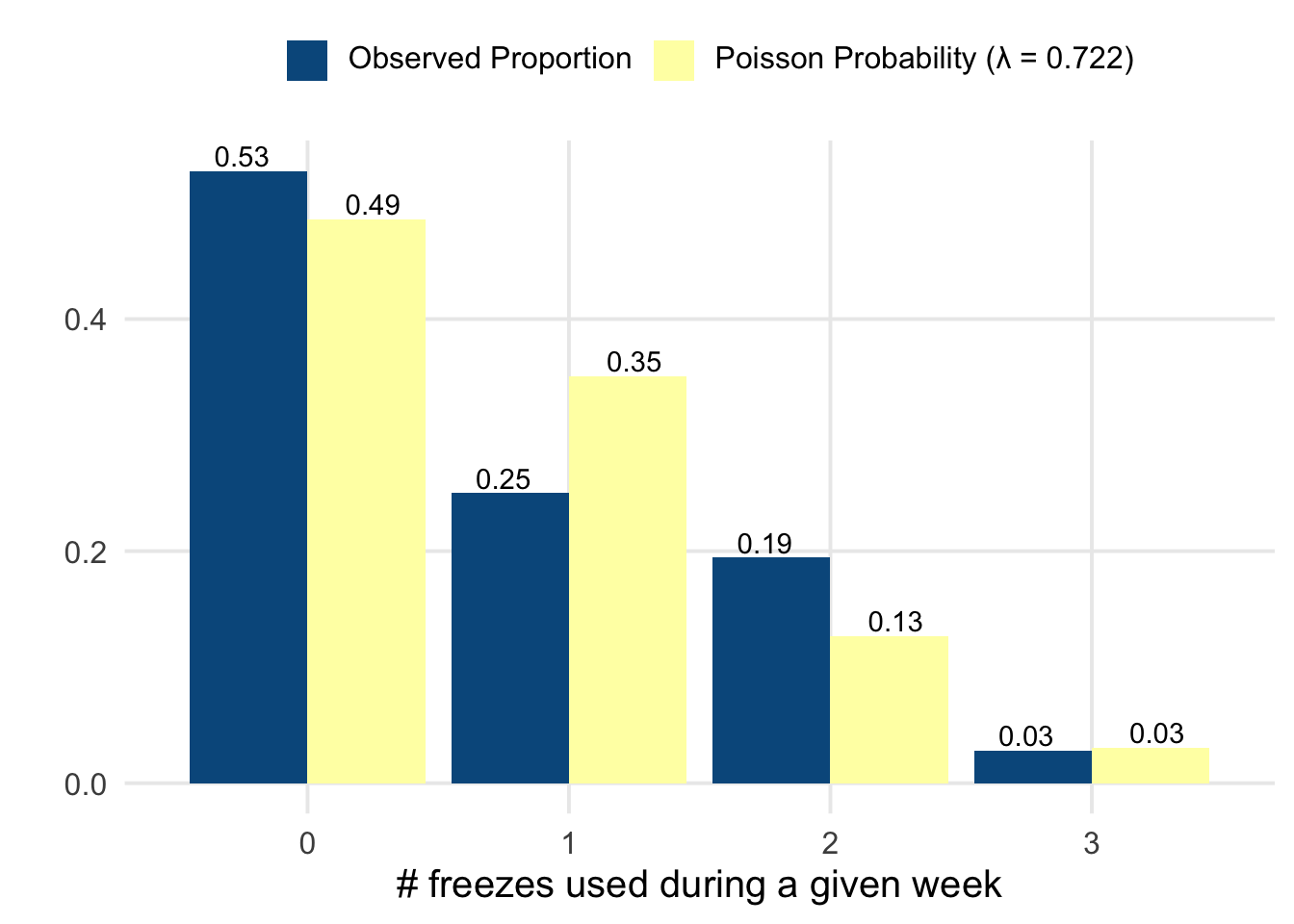

Maybe my data isn’t a perfect fit to a Poisson distribution with the same mean, but perhaps it’s close enough to serve as a model for what we can expect. So, to be specific, let’s let

\(X\) = the number of streak freezes used in a 7-day period, where \(X \sim Poisson(\lambda = 0.722)\).

We can then simulate 17 weeks from \(X\) and sum the results, repeating this process say, 10,000 times. Or, more formally, we end up with a vector of sums \(\vec{s}\):

\(\vec{s} = \begin{bmatrix}s_1 \\ s_2 \\ \vdots \\ s_j \end{bmatrix} \text{ where } j = 1, 2, 3, \cdots, 10,000, \text{ and } s_j = \sum_{i=1}^{17}[\vec{x}_i]\), if we let \(\vec{x}\) be the \(j^{th}\) sample from \(X\).

For this simulation, we’re assuming that the results of each week are independent of each other. This feels reasonable to me; autocorrelation in my tabulated weekly counts seems negligible.² All that’s left is to set up a loop to collect the simulation results, and then we’ll use a histogram to visualize them.

X <- Poisson(0.722)
s <- c()

for (b in 1:10000) {
  x <- random(X, n = 17)
  s <- c(s, sum(x))
}

ggplot(tibble(s), aes(x = s)) +
  geom_histogram(color = "white", bins = 15) +
  scale_y_continuous(labels = scales::comma) +
  theme(plot.caption = ggtext::element_markdown()) +
  labs(
    x = "Total # of simulated freezes observed over 17 weeks", y = "N",
    caption = str_glue(
      "*s*<sub>Mean</sub> = {round(mean(s), 2)}, *s*<sub>SD</sub> = {round(sd(s), 2)} ",
      "Pr(8 &le; *s* &le; 13) = {sum(between(s, 8, 13)) / length(s)}<br>",
      "Pr(7 &le; *s* &le; 21) = {sum(between(s, 7, 21)) / length(s)}"
    )
  )

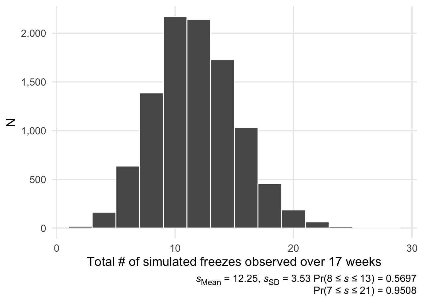
We end up with a fairly normal-looking histogram, as would be expected by the central limit theorem.³ If the model is appropriate, it seems like I should expect between 8 to 13 additional freezes to be accumulated over this time period. The simulation results suggest there’s only a 22% chance that the number of freezes accumulated will be less than 10. Pulling everything together, by the end of August I’ll probably be between 34 and 39 streak-freezes deep. This means it’ll be at least a month after my starting point before I can truly claim I’ve met my goal. 😭