This year, my partner has been working to complete her Masters in Natural Resources/Land Management, and several of her assignments have required some data analysis. One topic area we covered together was linear regression/multiple linear regression. As techniques, simple linear regression and multiple linear regression are well-known as workhorses for answering statistical questions across many scientific fields. Given their ubiquity, having the requisite working knowledge needed to interpret and evaluate a regression analysis is highly valuable in virtually any professional field that involves the use or consumption of data. This post is the first in a series, and I have a few objectives I hope to have met when they’re completed:
- Summarize the basic overview of linear regression I covered with my partner this year
- I’d like to have my notes in one place, and maybe placing them where others can find them would be useful
- Explain the minimal code needed to fit a regression model in R
- Introduce a few commonly-used R packages that can make interpreting and evaluating a regression model easier
For this series, I’m assuming you have a bit of exposure to the R language, ideally know how to make a plot with the {ggplot2} package, and can do some basic algebra. The focus of this post will be a big-picture overview of the mathematical problem that linear regression is attempting to solve, but one of the best resources I’ve encountered on the mechanics of regression is a blog post written by Chris Henson. Henson’s post is detailed (& a bit lengthy), but if you’re curious about the mathematical underpinnings of a regression analysis beyond what I discuss here, it might be of interest to you. Additionally, I don’t know if I’ll dedicate posts to this subject myself, but I’ve greatly appreciated Jonas K. Lindelov’s initial twitter thread and website that illustrates how common statistical techniques (such as t-tests, ANOVAs, correlations, etc.) are all linear models, drawing on a shared statistical framework.
motivation: outcomes & predictors
Fundamentally, linear regression is used when an analyst is interested in modeling the mean of a numeric & continuous outcome variable, based on one or more inputs (called predictor variables, or predictors)1. In our case, we’re going to wear the hat of an antarctic biologist, studying different characteristics of several different species of Penguins in the south pole. You can follow along, assuming you’ve installed the R language on your computer, and both the {tidyverse} and {palmerpenguins} packages.2
Let’s assume that the outcome we’re interested in is the bill lengths of the penguins we’re able to study in this region, such as the Gentoo (as depicted by @allison_horst).

For our research question, perhaps we’re interested in how well the length of a penguin’s bill can be predicted by the length of its flippers. We’ll start by visualizing this relationship as a scatterplot.
library(tidyverse)
library(palmerpenguins)

ggplot(data = penguins, aes(x = flipper_length_mm, y = bill_length_mm)) +
  geom_point() +
  labs(x = "Flipper Length (mm)", y = "Bill Length (mm)")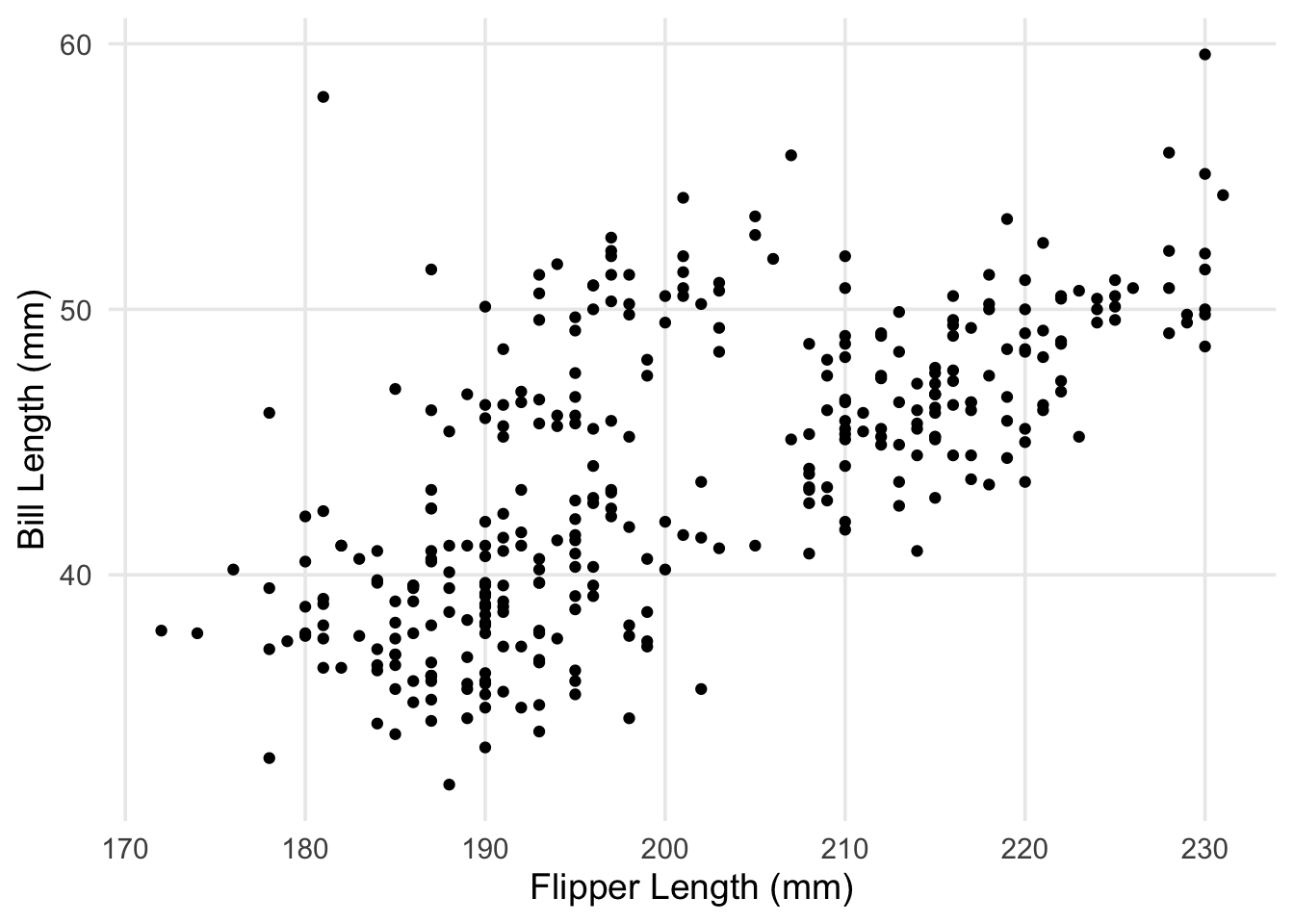
Right away, we can see a positive assocation; penguins with longer flippers tend to have longer bills. This is a good start, but if we wanted to summarize this association (or predict the bill lengths of penguins not in our data), we could try using a statistical model to do so. One of the simplest models we could use is a line, with the slope summarizing how bill length changes per 1-mm increase in flipper length. Fair enough, but how do we choose or specify which line to summarize the pattern in our data? Here’s our scatterplot again, but with a handful of candidate lines that we could draw through the points.
ggplot(penguins, aes(x = flipper_length_mm, y = bill_length_mm)) +
  geom_abline(slope = c(0.2548, 0.27, 0.23, 0.3818, 0.3), intercept = c(-7.2649, -7.43, -6.7, -31.31, -17.96), color = "blue") +
  geom_point() +
  labs(x = "Flipper Length (mm)", y = "Bill Length (mm)")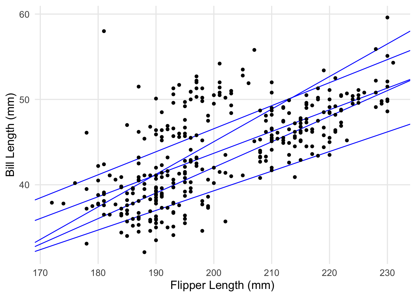
I made up each of these lines, and some might be better or worse for describing the association between the two variables. However, I could keep going, plotting 10, 20, 1000 lines, etc. There’s an infinite number that could be picked from! In practice, we need a method for choosing a line that’s best for the data we have, based on some reasonable criteria. This problem, narrowing down an infinite number of possible lines to one, is the task that linear regression attempts to solve.
an approach for finding the best line (OLS)
I’m now going to reference some equations, but they’re really just to clarify some commonly-used notation, and maybe jog your memory a little. In algebra, we learn that a line can be defined using two points in a plane (denoted \((x_1, y_1)\) and \((x_2, y_2)\)), resulting in an equation like this:
where m, the slope, is defined as \(m = \frac{(y_2-y_1)}{(x_2-x_1)}\) and b, the intercept, is \(b = y_1 - m(x_1)\). In my last plot, all I basically did was assemble and plot a bunch of these equations arbitrarily. However, the final product of a linear regression is also an equation, and despite the appearence of some Greek letters, I hope looks familiar:
This equation is our statistical model, and the terms \(\hat{\beta_0}\) and \(\hat{\beta_1}\) are the estimated intercept and slope of the proposed line to summarize our data (the little “hats” above each letter are used to indicate these are values estimated from data). The “betas” are also sometimes referred to as the parameters being estimated in a linear regression. On the left-hand side, \(y_i\) denotes the \(i\)-th bill length our line is attempting to predict (after accepting \(x_i\) as an input), while \(\epsilon_i\) on the right-hand side represents statistical noise (i.e. differences from the predicted line that are left over, and can’t be explained by our model3). So, how do we find estimates for \(\beta_0\) and \(\beta_1\)? One commonly used method is to choose values for \(\beta_0\) and \(\beta_1\) that minimize the results of this expression:
This is known as the sum of squared errors between each actual value of our outcome variable (\(y_i\)), versus the predicted value (\(\hat{y_i}\)) for that point generated by the model, where \(i\) ranges from 1 to the number of total data points (commonly denoted as n).4 In this post, we won’t go through the calculus required to show exactly how this happens, but a graphical explanation might be helpful.
ggplot(penguins, aes(x = flipper_length_mm, y = bill_length_mm)) +
  geom_abline(slope = 0.3, intercept = -17.96, color = "blue") +
  geom_segment(aes(y = (-17.96 + 0.3 * flipper_length_mm), yend = bill_length_mm, x = flipper_length_mm, xend = flipper_length_mm), color = "orange") +
  geom_point() +
  labs(x = "Flipper Length (mm)", y = "Bill Length (mm)")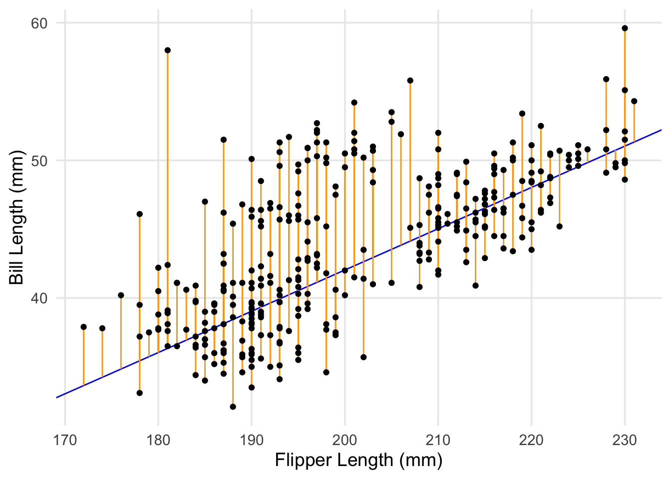
This is the same scatterplot we’ve been looking at, but now the differences (orange) between the points and one of my arbitrary lines (blue) have been emphasized. There are 344 penguins in our data, so we have a total of 344 differences between the actual points and any proposed line. Each of these differences are then squared and summed, with the algorithm working through values of \(\beta_0\) and \(\beta_1\) to search through possible lines until the minimum (i.e. the line with the smallest amount of error across all points) is identified.
So, to wrap up, some concluding remarks and takeaways:
In this post we focused on how linear regression works to fit a line between an outcome variable and a single predictor variable. This is often referred to as simple linear regression. However, as we’ll discuss later, you’re not restricted to conducting an analysis with only one predictor variable. Indeed, one of the strengths of linear regression is that it can be used to predict an outcome based on a combination of many different predictors within the same model.
The process of finding optimal values for \(\beta_0\) and \(\beta_1\) I’ve described is called Ordinary Least Squares (OLS), which takes its name from the quantity that’s minimized (i.e. the sum of squared errors). OLS is actually just one approach of many that’s been developed to estimate the parameters of a linear regression model. Although this wasn’t explicitly stated in my overview, the approach depends on calculating the means for the outcome variable and predictor variable(s), but there are other variations that e.g. rely on predictor/outcome medians.
We didn’t cover common assumptions that one should attend to when evaluating whether a linear regression will provide useful or valid results. These are important to consider, and we’ll discuss some of them more deeply in part 2. In the context of what we’ve discussed here, the most important consideration is whether the predictor variables you’re analyzing can be expected to have a linear relationship with your outcome.
- Specifically, you’re assuming that an increase/decrease of 1 unit of your predictor would result in the same amount of change in your outcome variable, across the entirety of the predictor’s range. In practice, this assumption isn’t always strictly met by real-world data. However, it’s important to understand that this is a built-in aspect of how linear regression “sees” the world. In some cases, transforming certain predictors (e.g. applying a square-root or log function to them) can be beneficial, but thinking about what you’re actually asking from a model is important. I’ve found Richard McElreath’s likening the pitfalls that statistical models can have to the story of the golem of Prauge to be helpful for thinking about this issue.
In the next post, we’ll cover the lm() function used to fit linear regression models in R, how to use basic diagnostic plots to check whether your model is performing well, and how to extract different estimates of interest from model objects. I hope you found this useful & informative! There are an abundance of good resources for learning about linear regression as a technique, but many of us are exposed to things in piecemeal fashion or find ourselves having to relearn concepts long after we first encounter them. I’ve found value in seeing this topic described in different ways and by different authors, so perhaps my overview can be a useful stepping stone on whatever journey you’re taking.
Under some conventions, you may have seen the the outcome and predictors being referred to as a dependent variable and independent variables. I prefer outcome/predictor, as the roles being played by each term feel slightly more intuitive to me.↩︎
Everything needed can be fetched from CRAN; in your console, you can run
install.packages("tidyverse")andinstall.packages("palmerpenguins")to ensure both are available for R to use.↩︎We won’t discuss this in detail here, but this is a point to mention one of the commonly noted assumptions of linear regression, i.e. that these errors, \(\epsilon\), come from a specific distribution (normal/Gaussian), and don’t systematically vary across the data used in the model.
↩︎Note that what’s written as \(\hat{y_i}\) in the expression can be expressed as \((y_i - \hat{\beta_0} - \hat{\beta_1}{x_i})^2\)↩︎