This is a continuation from a previous post, which can be found here. Okay, picking up where we left off! In this post we’ll dive into building a set of models that can classify each of my playlist tracks as a “top-song” or not. While this is an exploration of some boutique data, it’s also a cursory look at many of the packages found in the tidymodels ecosystem. A few posts I found useful in terms of working with tidymodels can be found here, and here.
processing & training
We’ll start by setting up our environment, and pulling in the data analyzed in part 1. While I don’t always feel the need to detail everything going on in this step, there are two extra-crucial commands right at the top. The first is set.seed(). For my own sanity, I want to make sure that small differences due to random chance aren’t changing as I work on the models/analysis. We’ll be using k-fold cross validation (which involves randomly splitting a dataset into k equal parts) and boostrap resampling, both of which will need a seed specified (if we want the results to be reproducible). The next is an options() call– the yardstick package typically treats the first level of categorical variables as the target level. For dichotomous outcomes I’m used to treating 0 as negative and 1 as positive, and it feels right to keep them in order. If you’re like me, it’s important to toggle this option so your metrics are calculated correctly!
set.seed(20190914)
options(yardstick.event_first = FALSE)

library(tidyverse)
library(tidymodels)
library(zeallot)

theme_set(
  theme_minimal(base_size = 20) +
    theme(
      panel.grid.minor = element_blank(),
      axis.text        = element_text(face = "bold")
    )
)

tracks <- read_csv("../../static/data/predicting-top-songs/20190915-ts-tracks-train-test.csv")
Here we’ll do some minor setup based on our results from the previous post. I wanted to create a 4-level variable with the key/mode combination for each track, based on how likely they were to end up in one of my “top songs” playlists.
# prepare the key/mode and season variables we explored in part 1
tracks <- tracks %>%
  mutate(
    is_target     = factor(is_target),

    keygroup = case_when(
      key_mode %in% c(
        "D# minor", "B major", "G minor", "C minor", "A# major"
      ) ~ "great",
      key_mode %in% c(
        "C# minor", "F# major", "A major", "D minor", "G major", "A minor",
        "C major"
      ) ~ "good",
      key_mode %in% c(
        "E minor", "A# minor"
      ) ~ "not good",
      TRUE ~ "fine"
    )
  )
Next, we’ll set up our training and test data that we generated in part 1. Instead of just building models with our training set alone, I want to average out the performance using a cross-validation technique: K-fold (or V-fold) cross validation. There are several resources that explain in greater detail what K-fold CV is and why you should use it, so I won’t dive into it here. The super abbreviated explanation is that the data is split into k different parts; \(k-1\) of the parts are used to build a model, and the final partition is held out for the model to predict. Each possible combination of splits is used to train the model, and afterwards the model’s average performance can be computed across the k different attempts.
# break out the training/test set into different frames, and drop some unused variables
tracks <- tracks %>%
  split(tracks$dataset) %>%
  map(~select(., -dataset, -time_signature, -playlist_name, -playlist_img))

# zeallot's multi-assignment operator that can be used to unpack lists cleanly
c(test, train) %<-% tracks

ts_cvdat <- vfold_cv(train)
Because we’ll be building models on a buch of different datasts, we need to define functions that will apply the same processing instuctions each time. The first function will hold the recipe for each model that we’ll train. Recipes (recipes::recipe()) describe outcome and predictor variables in a dataset, as well as processing steps that need to be applied before building a model. In the code block below, you’ll see a few things happening:
- A formula for the recipe is specified; the variable on the left-hand side will be treated as the outcome/dependent variable in the data being operated on, while the variables on the right-hand side will be treated as predictors.
- A chain of steps is specified, with options being controlled by arguments from the function we’re defining.
recipes::step_upsample()allows us to resample the target class, so that the class represented more frequently post-processing.- In our dataset, the outcome is fairly imbalanced (only 23.7% of our tracks ended up as a top-song). Classifiers often have difficulties when classes aren’t represented evenly, so upsampling may help partially skirt this issue. Downsampling (i.e. randomly discarding cases from the non-target class) is also an option for dealing with imbalanced data, but we really don’t have too many tracks to begin with, so retaining all of them seems to be the best route.
- Importantly, upsampling is something that should only be applied during model training. This is why we’re controlling the step with the
skip_toggleargument in our function. When validating our models, we want to make sure that they perform well on data as it would exist in the wild. The imbalanced nature of our data is a part of the context from which they were drawn, so we want to make sure that’s preserved when we evaluate performance.
recipes::step_dummy()is a bit simpler. All this does is generate dummy (binary 0/1) columns for each of our categorical variables (while automatically excluding a reference category).- Note that I’m referring to column names as I would when using
dplyr::select(). Much like the tidyverse, packages in tidymodels use Non-Standard Evaluation, making specifying commands familiar for folks already familiar with dplyr et al.
- Note that I’m referring to column names as I would when using
ts_recipe <- function(dataset, skip_toggle = TRUE, r = .7) {
  # the full formula of variables to be included for modeling
  f <- is_target ~ keygroup + playlist_mon

  # up-sample our target class in order to even out the class imbalance
  # with our specified variables, create dummies for the year/mon and keygroup
  recipe(f, data = dataset) %>%
    step_upsample(is_target, ratio = r, skip = skip_toggle) %>%
    step_dummy(keygroup, playlist_mon)
}
The recipes package has a ton of other step_ functions, with commands that can handle things like centering/scaling, imputation of missing data, and principle components analysis (just to name a few). There’s even a textrecipes package that I’ve been curious about, which extends the framework to analysis of text-based data. Most of the common steps that one has to take in terms of preparing a pipeline for processing data prior to modeling are well-covered, and this little example just scratches the surface.
Now that we’ve specified how we want to preprocess the data, we can set up master functions that will be applied to each split in our training data. Just to briefly cover what this next function is doing:
- It accepts a
splitgenerated from avfold_cvobject, and uses theanalysis()andassessment()functions to extract the datasets. - The recipe we defined above is
prep()’d andbake()’d (i.e. the processing steps are applied based on the provided recipe, and processed datasets are generated). - Using functions from the parsnip package, we create a model object, using a specific model engine, and specify a model fit based on the variables in our dataset.
- In this case we’re setting up a logistic regression, with the goal of classification, using
stats::glm().
- In this case we’re setting up a logistic regression, with the goal of classification, using
- Lastly, we predict the classification of each case in our validation/assessment data, and return the predictions as a tibble.
ts_logit <- function(split, id, r = .7) {
  # extract the analysis/assessment sets from the split
  tr <- analysis(split)
  ts <- assessment(split)

  # prep/bake the data according to the recipe
  # the *r* argument controls how much the target class should be upsampled
  # an *r* of 1 means both classes should be the same size
  tr_prep <- prep(ts_recipe(tr, skip_toggle = FALSE, r = r), training = tr)
  tr_proc <- bake(tr_prep, new_data = tr)

  ts_prep <- prep(ts_recipe(ts), testing = ts)
  ts_proc <- bake(ts_prep, new_data = ts)

  # build the model with the prepped analysis set
  model <- logistic_reg("classification") %>%
    set_engine("glm") %>%
    fit(is_target ~ ., data = tr_proc)

  # apply the model to the assessment set, and return a tibble
  tibble(
    `id`  = id,
    truth = ts_proc$is_target,
    pred  = unlist(predict(model, ts_proc))
  )
}
I’ve only showed one model as an example, but I’ve used the same framework to set up a random forest classifier, a KNN classifier, and a final function that stacks all 3 of the individual classifiers, and builds a random forest using the other models’ predictions as additional features. This is an additional ensemble technique that I’ll discuss when we’ll get to the results.
Now, all that’s left is to train the models and evaluate them! Given that all the analysis has been defined in some smaller functions, we can just loop over each split with purr::map2_df() to create tibbles with predictions from each split for each different model.
lr  <- map2_df(.x = ts_cvdat$splits, .y = ts_cvdat$id, ~ts_logit(.x, .y))
rf  <- map2_df(.x = ts_cvdat$splits, .y = ts_cvdat$id, ~ts_rf(.x, .y))
knn <- map2_df(.x = ts_cvdat$splits, .y = ts_cvdat$id, ~ts_knn(.x, .y))

# the stacked model results
stacked_res <- map2_df(.x = ts_cvdat$splits, .y = ts_cvdat$id, ~ts_stacked(.x, .y))
evaluation
Let’s see how well we did. Given that our outcome variable is binary, a lot of the metrics we’ll be using to evaluate the performance of each model may be familiar, and can be easily conceptualized using a confusion table, like the one below:
| Predicted/Reference | Positive | Negative |
|---|---|---|
| Positive | A | B |
| Negative | C | D |
Specifically, we’ll be using the following:
Accuracy = (A + D) / (A + B + C + D)
- The metric that most folks are familiar with, i.e the proportion of all cases that were predicted correctly.
Sensitivity = A / (A + C)
- Also known as “recall”, this metric represents the proportion of positive cases that were correctly predicted.
Specificity = D / (B + D)
- This metric represents the proportion of negative cases that were correctly predicted.
Balanced Accuracy = mean(Sensitivity, Specificity)
- This is merely an average of sensitivity and specificity.
Kappa = \(1 - \frac{1-p_0}{1-p_E}\) (where \(p_0\) is the observed agreement, and \(p_E\) is the expected agreement due to chance)
- Similar to accuracy, but adjusts to account for agreement based on chance alone. Often helpful when classes are imbalanced (e.g. in this context).
Each one of these measures can be computed using a function from yardstick, e.g. spec() and sens(), which accept a tibble/data.frame and expect columns representing predictions and actual class values (in the case of classification). We can create a special list for each of our metrics using yardstick::metric_set(), and then apply each of them to columns in a tibble. Handily, you can use a metric set in tandem with group_by(), which enables us to concisely summarize performance across all the folds/models. Let’s take a peek at the median performance for each model using a bar plot. Also note that each of these measures range from 0 to 1, with 1 representing the highest performance.
class_metrics <- metric_set(sens, spec, accuracy, kap, bal_accuracy)

train_cv_results <-
  bind_rows(LR = lr, RF = rf, KNN = knn, Agg = stacked_res, .id  = "model") %>%
  group_by(model, id) %>%
  class_metrics(truth = truth, estimate = pred) %>%
  group_by(model, .metric) %>%
  summarise_at(vars(.estimate), list(median, mean, sd))

# bar plot with median values for each metric
p_train_metrics <- train_cv_results %>%
  select(-fn2, -fn3) %>%
  gather(desc, val, fn1) %>%
  mutate(
    .metric = fct_recode(
      .metric,
      Accuracy            = "accuracy",
      `Balanced Accuracy` = "bal_accuracy",
      Kappa               = "kap",
      Specificity         = "spec",
      Sensitivity         = "sens"
    ),
  ) %>%
  ggplot(aes(x = .metric, y = val, fill = model)) +
  geom_col(position = "dodge") +
  scale_fill_manual("Model", values = scico::scico(4, palette = "nuuk")) +
  labs(x = "", y = "Median across 10 folds") +
  theme(legend.position = "top")

p_train_metrics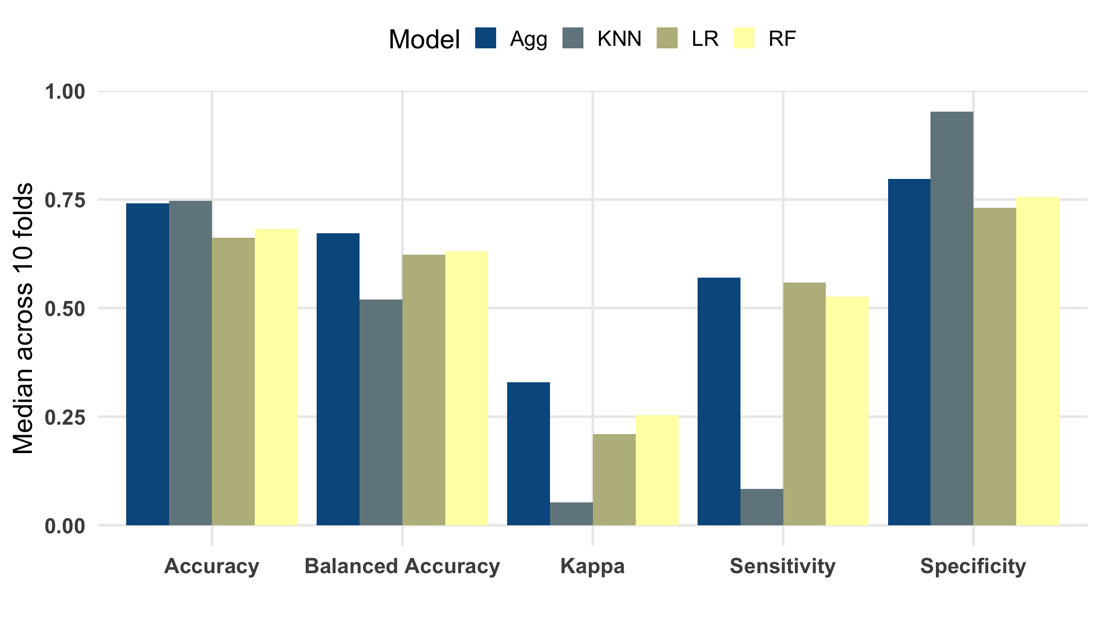
So, the picture from our training data? Fine, but not great! One of the things that’s clear is that the individual classifiers have some different strengths. First, the KNN classifier appears to have the highest overall accuracy, but this is driven almost entirely to classify non top-song tracks correctly. You can see this based on its rank within specificity and sensitivity. I experimented with varying the number of nearest-neighbors from 0-12, and 4 seemed best on-balance. Second, the random forest classifier seemed to trail a bit behind the logistic regression, although they’re mostly comparable. Increasing the number of trees in the forest past a few thousand didn’t really provide much of a boost. Lastly, the stacked/aggregated classifier appears to have done a fair amount better than any of the models on their own. My hopes were that I could borrow some of the specificity from the KNN classifier, while retaining sensitivity from the logit and RF models, and it seems to have paid off. Even still, we’re only correctly classifying just over half of all true top-songs, and 75% of non top-songs.
Now, for a final test with our holdout data. The stacked/aggregated model seems to be our best performer, so we’ll refit the model using all of our available training data, and predict all of the cases left in our holdout data.
| Accuracy | Balanced Accuracy | Kappa | Sensitivty | Specificity |
|---|---|---|---|---|
| 0.68 | 0.59 | 0.16 | 0.43 | 0.75 |
Oof, worse on all accounts. Guess we’re dealing with some overfitting. Well, this certainly isn’t a glittering example of artificial intelligence, but I think it’s pretty cool to get this far mostly by knowing a track’s key/mode. Maybe there are some other things that I’ve annotated or haven’t thought of that can help predict things a bit better. Just a little over 1.5 months until December, so maybe I’ll loop back if something strikes me, and either update this post with the results for 2019, or spin off what I find into a new post.